Frequent Symptom Mining – MaineR Users Group

Quotes

“In God we trust, all others bring data.” - W. Edwards Deming
“Data mining is not about finding the right answers, it’s about asking the right questions.” - Anonymous
“Data mining is the process of finding needles in haystacks, and then finding the other needles that are hidden in those needles.” - Anonymous
“You didn’t know? You better call somebody!” - Road Dogg, WWE

Outline

Background of the Problem
Background of the Method
R packages
Basic example(s)
The crux of the matter
Symptom mining

Disclosure

Background of the Problem

Neonatal Abstinence Syndrome (NAS)

In utero opiod exposure
Characterized by withdrawal symptoms
ICD-9 779.5
ICD-10 P96.1
Number of diagnoses increasing
Control costs (lengthy stays)
Detection is essential for health of infant
Treatment is pharmacological therapy with morphine, methadone, or phenobarbital

Finnigan NAS Score (FNASS)

21 symptoms scored
5 gastronintesinal (e.g., vomit)
7 Centrial nerous system (e.g., tremors)
9 Respiratory (e.g., stuffiness, flaring)
Scored every 4 hours
Many scoring systems
- Lipsitz (Lipsitz, 1975)
- Neonatal Withdrawal Inventory (Zahorodny et al., 1998)
- FNASS (Finnegan et al., 1975)

Goal

Reduce the number of items
ESC (Curran et al., 2020)
Mine frequent (assocaiated) symptoms

Research Team

Tina Holt, M.D., Maine Medical Center
Meg Curran, M.D., Maine Medical Center
Michael Arciero, Ph.D. University of New England
Curran, M., Holt, C., Arciero, M., Quinlan, J., Cox, D., & Craig, A. (2020). Proxy Finnegan component scores for eat, sleep, console in a cohort of opioid-exposed neonates. Hospital Pediatrics, 10(12), 1053-1058.

Background of the Method

Itemset & Rule Mining

Find (useful) patterns in a database
Frequent co-occurrence
Frequent Itemset Mining
Sequence Mining
Market Basket Analysis
- Modern parlance

Applications

Retail sales (MBA)
Web usage (data information brokers)
Congressional Voting Records
Law enforcement profiling
Recommender systems
Supply chain analysis
Extract information hidden in DNA sequences
Gene ontology
Concussion symptims (sleep, light sensitivity)

Terminology

Items are denoted by \(\mathcal{I} = \{i_1, i_2, \dots, i_n \}\) and transactions (a.k.a. events, observations, records) as \(T = \{t_1, t_2, \dots, t_N\}\) where \(N > n\) and \(N \gg 1\).
- “Items” are symptoms in our case
Itemset is any group of one or more items, also called basket or cart.
- e.g., \(X = \{ i_3, i_{17}, i_{1325} \}\)
Frequent item set is an itemset that meets (some) criteria.
Let \(X\) be a subset of items, then the support count is the number of transactions containing \(X\). [ { (X) = | {t_i | X t_i T }| } ]
Association Rule is an implication of the form \(X \Rightarrow Y\) where \(X \cap Y = \emptyset\).

Measures of Strength and Interest

The following measure the strength of an association or frequency of an itemset.

The support (how often the rule applies) \[ \large{ S(X \Rightarrow Y) = \frac{\sigma(X \cup Y)}{N} } \] where \(N\) is the total number of transactions in the database.

Confidence how frequently items in \(Y\) appears in transactions that contain \(X\).
\[ \large{ C(X \Rightarrow Y) = \frac{\sigma(X \cup Y)}{\sigma(X)} } \]
Lift (Brin et al., 1997), ratio of combined support from expected independence \[ \large{ L(X \Rightarrow Y) = \frac{ N \sigma(X \cup Y)}{\sigma(X) \cdot \sigma(Y)} = \frac{C(X,Y)}{S(Y)} } \]

Example

1	Milk	Eggs	Diapers	Beer
2	Milk		Diapers
3		Eggs	Diapers	Beer
4	Milk	Eggs
5	Milk		Diapers	Beer

Consider the transaction database with \(X = \{ \text{Diapers} \}\) and \(Y = \{\text{Beer}\}\).

Support, \(S(X,Y) = 3/5 = 0.6\)
Confidence, \(C(X,Y) = 3/4 = 0.75\)
Lift, \(L(X,Y) = (5 \cdot 3) / (4 \cdot 3) = 1.25\)

Binary Database

tid	Milk	Eggs	Diapers	Beer
1	1	1	1	1
2	1	0	1	0
3	0	1	1	1
4	1	1	0	0
5	1	0	1	1

Rule Mining / Itemset Selection

Frequent item set is an itemset that meets minimum support criteria.
Given \(d\) items, exclude the \(0\) element set and the \(d\) element set.
For each subset \(k\)-element subset \(X\), we consider the \(d-k\) element subsets \(Y\). [ {k = 1}^{d-1} {i = 1}^{d-k} = 3^d - 2^{d+1} + 1 ]
Brute force is computationally prohibitive
- Exponential time, \(O(3^d)\)
Subset reduction needed
- Apriori Algorithm

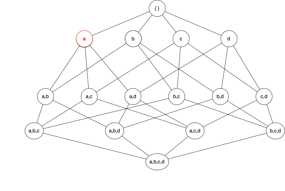
Aprior Algorithm

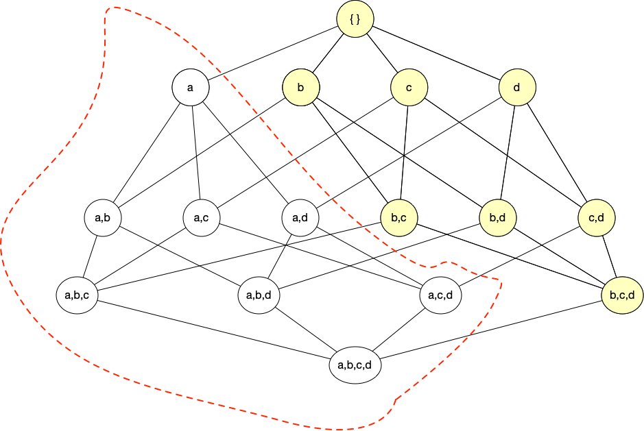
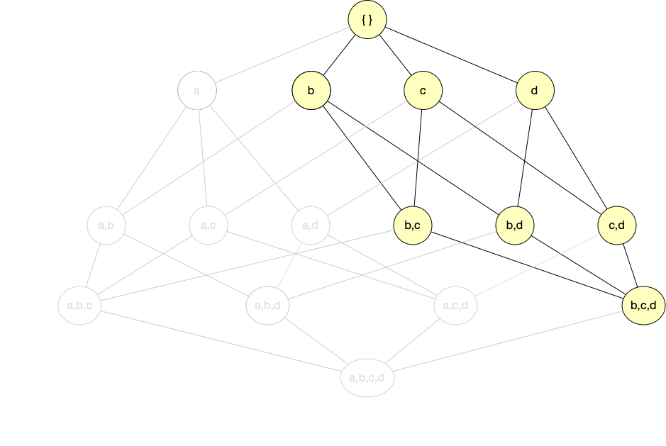
Apriori Principle: If an itemset is frequent, then all its subsets are frequent.
Contrapositive: If a subset is infrequent, then all its supersets are infrequent.

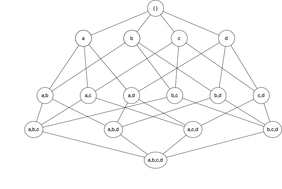
Compact representations

Definition - A frequent itemset is maximal if none of its immediate supersets are frequent.

All frequent itemsets are a subset of the maximal itemsets.

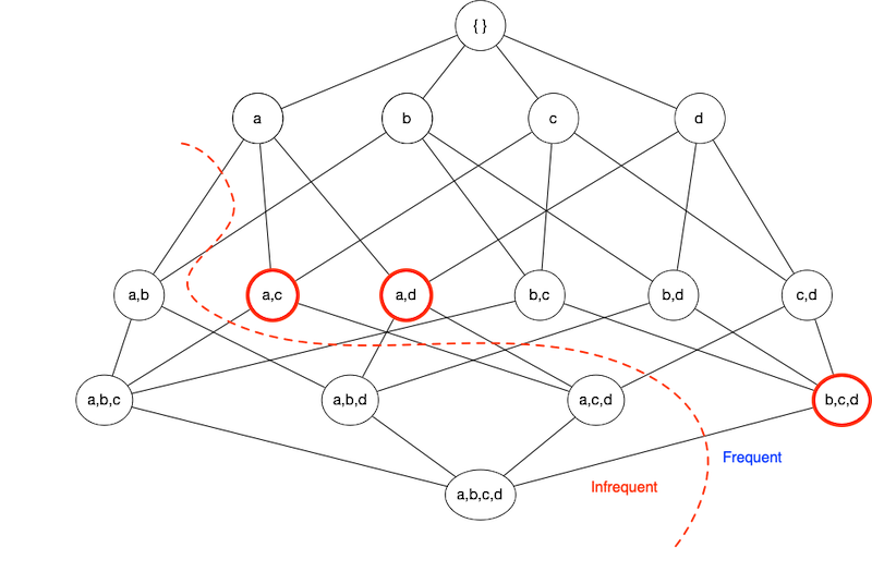
Compact representations (cont)

Definition - An itemset \(X\) is closed if none of its immediate supersets has exactly the same support count as \(X\). An itemset is a closed frequent itemset if it is closed and its support is greater than or equal to minimum support.

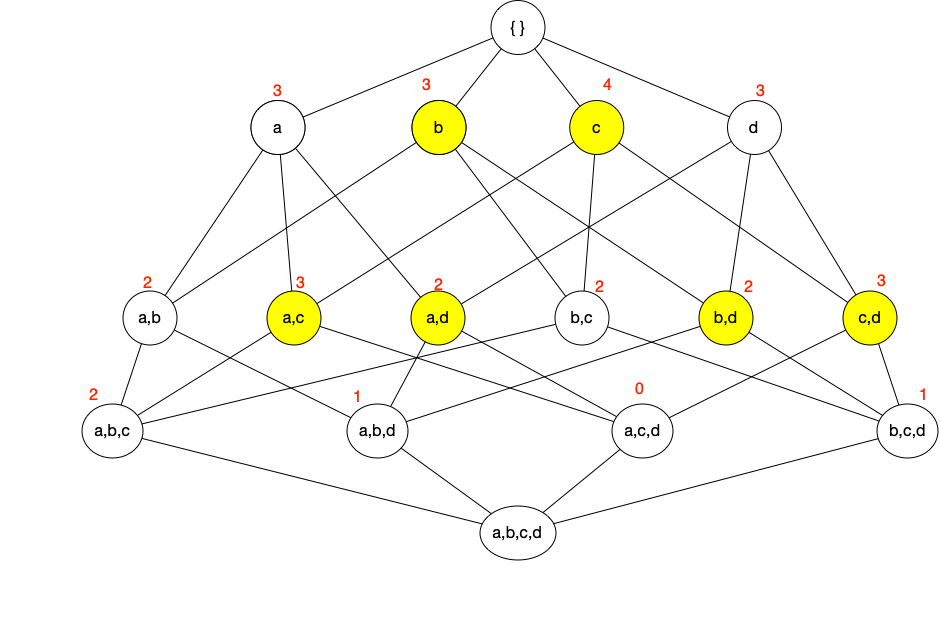
Compact Representation Diagram

R packages

aRules - Mining Association Rules and Frequent Itemsets
- Apriori and eclat algorithms
aRulesViz - Visualize Association Rules
arulesSequences - Mining Frequent Sequences
tidyverse - Tidy ecosystem

Install and Load

# install.packages("tidyverse")
# install.packages("arules")
# install.packages("arulesViz")
# install.packages("arulesSequences")

library(tidyverse)
library(arules)
library(arulesViz)
library(arulesSequences)

aRules 1.7-5

inspect - display rules in readable form
itemFrequency - Frequency/Support for Single Items
itemMatrix - building block for transactions
apriori - Mine frequent itemsets, association rules
eclat - Mine frequent itemsets with the Eclat algorithm.
- equivalence class clustering along with bottom-up lattice traversal.
transactions - subclass of itemMatrix. Note: Data typically starts as a data.frame or a matrix and needs to be prepared before it can be converted into transactions
Read the Manual
- https://cran.r-project.org/web/packages/arules/arules.pdf
Check dependencies (e.g., Matrix \(\ge\) 1.4)

Example

# Load Example Data (from aRules package)
data("Groceries")
class(Groceries)

[1] "transactions"
attr(,"package")
[1] "arules"

head(as(Groceries, "data.frame"), 10)

                                                                    items
1                {citrus fruit,semi-finished bread,margarine,ready soups}
2                                          {tropical fruit,yogurt,coffee}
3                                                            {whole milk}
4                           {pip fruit,yogurt,cream cheese ,meat spreads}
5   {other vegetables,whole milk,condensed milk,long life bakery product}
6                        {whole milk,butter,yogurt,rice,abrasive cleaner}
7                                                            {rolls/buns}
8  {other vegetables,UHT-milk,rolls/buns,bottled beer,liquor (appetizer)}
9                                                            {pot plants}
10                                                   {whole milk,cereals}

freqItems <- apriori(Groceries, 
                 parameter = list(
                   supp   = 0.01, 
                   conf   = 0.5, 
                   target = "frequent itemsets", 
                   minlen = 3, 
                   maxlen = 5)
                 )

Apriori

Parameter specification:
 confidence minval smax arem  aval originalSupport maxtime support minlen
         NA    0.1    1 none FALSE            TRUE       5    0.01      3
 maxlen            target  ext
      5 frequent itemsets TRUE

Algorithmic control:
 filter tree heap memopt load sort verbose
    0.1 TRUE TRUE  FALSE TRUE    2    TRUE

Absolute minimum support count: 98 

set item appearances ...[0 item(s)] done [0.00s].
set transactions ...[169 item(s), 9835 transaction(s)] done [0.00s].
sorting and recoding items ... [88 item(s)] done [0.00s].
creating transaction tree ... done [0.00s].
checking subsets of size 1 2 3 4 done [0.00s].
sorting transactions ... done [0.00s].
writing ... [32 set(s)] done [0.00s].
creating S4 object  ... done [0.00s].

head(as(freqItems,"data.frame") %>% arrange(desc(count)),10)

                                              items    support count
1     {root vegetables,other vegetables,whole milk} 0.02318251   228
2              {other vegetables,whole milk,yogurt} 0.02226741   219
3          {other vegetables,whole milk,rolls/buns} 0.01789527   176
4      {tropical fruit,other vegetables,whole milk} 0.01708185   168
5                    {whole milk,yogurt,rolls/buns} 0.01555669   153
6                {tropical fruit,whole milk,yogurt} 0.01514997   149
7  {other vegetables,whole milk,whipped/sour cream} 0.01464159   144
8               {root vegetables,whole milk,yogurt} 0.01453991   143
9                {other vegetables,whole milk,soda} 0.01392984   137
10          {pip fruit,other vegetables,whole milk} 0.01352313   133

rules <- apriori(Groceries, 
                 parameter = list(
                   supp   = 0.01, 
                   conf   = 0.5, 
                   target = "rules", 
                   minlen = 1, 
                   maxlen = 10)
                 )

head(as(rules,"data.frame") %>% arrange(desc(count)))

                                                  rules    support confidence
1             {other vegetables,yogurt} => {whole milk} 0.02226741  0.5128806
2               {tropical fruit,yogurt} => {whole milk} 0.01514997  0.5173611
3 {other vegetables,whipped/sour cream} => {whole milk} 0.01464159  0.5070423
4              {root vegetables,yogurt} => {whole milk} 0.01453991  0.5629921
5          {pip fruit,other vegetables} => {whole milk} 0.01352313  0.5175097
6        {root vegetables,yogurt} => {other vegetables} 0.01291307  0.5000000
    coverage     lift count
1 0.04341637 2.007235   219
2 0.02928317 2.024770   149
3 0.02887646 1.984385   144
4 0.02582613 2.203354   143
5 0.02613116 2.025351   133
6 0.02582613 2.584078   127

summary(rules)

set of 15 rules

rule length distribution (lhs + rhs):sizes
 3 
15 

   Min. 1st Qu.  Median    Mean 3rd Qu.    Max. 
      3       3       3       3       3       3 

summary of quality measures:
    support          confidence        coverage            lift      
 Min.   :0.01007   Min.   :0.5000   Min.   :0.01729   Min.   :1.984  
 1st Qu.:0.01174   1st Qu.:0.5151   1st Qu.:0.02089   1st Qu.:2.036  
 Median :0.01230   Median :0.5245   Median :0.02430   Median :2.203  
 Mean   :0.01316   Mean   :0.5411   Mean   :0.02454   Mean   :2.299  
 3rd Qu.:0.01403   3rd Qu.:0.5718   3rd Qu.:0.02598   3rd Qu.:2.432  
 Max.   :0.02227   Max.   :0.5862   Max.   :0.04342   Max.   :3.030  
     count      
 Min.   : 99.0  
 1st Qu.:115.5  
 Median :121.0  
 Mean   :129.4  
 3rd Qu.:138.0  
 Max.   :219.0  

mining info:
      data ntransactions support confidence
 Groceries          9835    0.01        0.5
                                                                                                            call
 apriori(data = Groceries, parameter = list(supp = 0.01, conf = 0.5, target = "rules", minlen = 1, maxlen = 10))

inspect(rules[1:10], by ="lift")

     lhs                                       rhs                support   
[1]  {curd, yogurt}                         => {whole milk}       0.01006609
[2]  {other vegetables, butter}             => {whole milk}       0.01148958
[3]  {other vegetables, domestic eggs}      => {whole milk}       0.01230300
[4]  {yogurt, whipped/sour cream}           => {whole milk}       0.01087951
[5]  {other vegetables, whipped/sour cream} => {whole milk}       0.01464159
[6]  {pip fruit, other vegetables}          => {whole milk}       0.01352313
[7]  {citrus fruit, root vegetables}        => {other vegetables} 0.01037112
[8]  {tropical fruit, root vegetables}      => {other vegetables} 0.01230300
[9]  {tropical fruit, root vegetables}      => {whole milk}       0.01199797
[10] {tropical fruit, yogurt}               => {whole milk}       0.01514997
     confidence coverage   lift     count
[1]  0.5823529  0.01728521 2.279125  99  
[2]  0.5736041  0.02003050 2.244885 113  
[3]  0.5525114  0.02226741 2.162336 121  
[4]  0.5245098  0.02074225 2.052747 107  
[5]  0.5070423  0.02887646 1.984385 144  
[6]  0.5175097  0.02613116 2.025351 133  
[7]  0.5862069  0.01769192 3.029608 102  
[8]  0.5845411  0.02104728 3.020999 121  
[9]  0.5700483  0.02104728 2.230969 118  
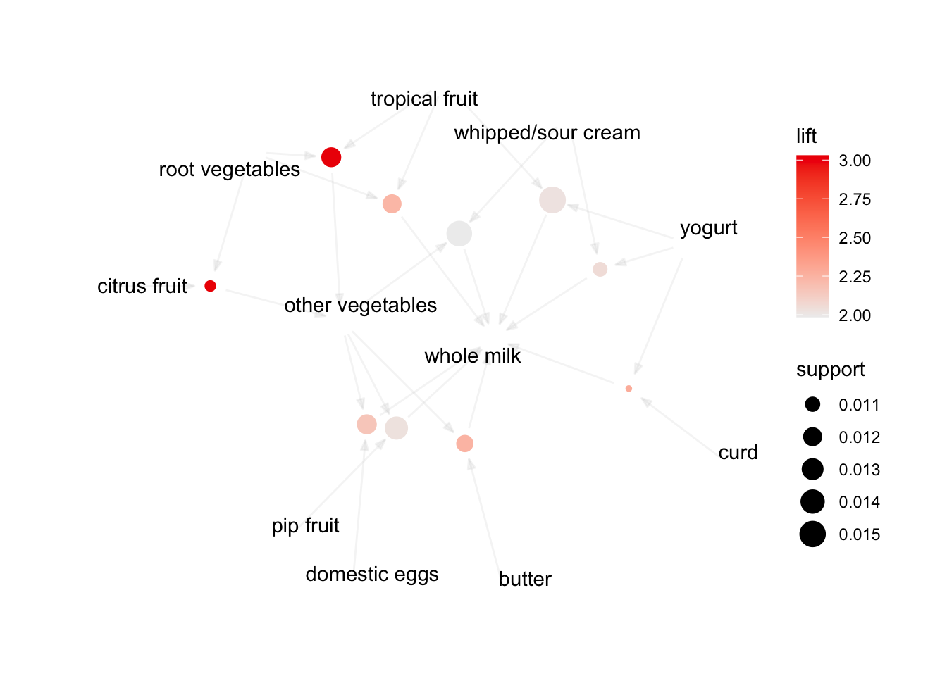
[10] 0.5173611  0.02928317 2.024770 149

`arulesViz` 1.5-2

Visualizing Association Rules and Frequent Itemsets

https://cran.r-project.org/web/packages/arulesViz/arulesViz.pdf
plot(rules, method="graph")
See also ggraph package for graph and network visualizations

plot(rules[1:10], method = "graph")

Frequent Sequences

Mining frequent sequential patterns with the cSPADE algorithm

SPADE (Sequential PAttern Discovery using Equivalence classes)
Temporal transactions (grouped by customer)
“If a customer buys \(X\) then in the next purchase will they buy \(Y\)”?
Web logs (\(a \to b \to c \to d\))
arulesSequences 0.2-28
cspade(transactions)

# create binary matrix of items
data <- data.frame(sequenceID = as.factor(c(1, 1, 1, 1, 2, 2, 3, 4, 4, 4)),
                   eventID = as.factor(c(1, 2, 3, 4, 1, 1, 1, 1, 2, 3)),
                   A = c(0, 1, 1, 1, 1, 0, 1, 0, 0, 1),
                   B = c(0, 1, 1, 0, 1, 0, 1, 0, 1, 0),
                   C = c(1, 1, 0, 1, 0, 0, 0, 0, 0, 0),
                   D = c(1, 0, 0, 0, 0, 0, 0, 1, 0, 0),
                   E = c(0, 0, 0, 0, 0, 1, 0, 0, 0, 0),
                   F = c(0, 0, 1, 1, 1, 0, 1, 0, 0, 1),
                   G = c(0, 0, 0, 0, 0, 0, 0, 1, 1, 0),
                   H = c(0, 0, 0, 0, 0, 0, 0, 1, 0, 1))

db <- pivot_longer(data, cols = c(3,4,5,6,7,8,9,10)) %>% filter(value > 0)

sequences <- db %>%
  group_by(sequenceID, eventID) %>%
  summarize(
    SIZE = n(),
    items = paste(as.character(name), collapse = ';')
  )

`summarise()` has regrouped the output.
ℹ Summaries were computed grouped by sequenceID and eventID.
ℹ Output is grouped by sequenceID.
ℹ Use `summarise(.groups = "drop_last")` to silence this message.
ℹ Use `summarise(.by = c(sequenceID, eventID))` for per-operation grouping
  (`?dplyr::dplyr_by`) instead.

names(sequences) = c("sequenceID", "eventID", "SIZE", "items")

sequences <- data.frame(lapply(sequences, as.factor))
sequences <- sequences[order(sequences$sequenceID, sequences$eventID),]

# Convert to transaction matrix data type
write.table(sequences, "seqs.txt", sep=";", row.names = FALSE, col.names = FALSE, quote = FALSE)
trans_matrix <- read_baskets("seqs.txt", sep = ";", info = c("sequenceID","eventID","SIZE"))

s1 <- cspade(trans_matrix, parameter = list(support = 0.6, maxlen=5), control = list(verbose = TRUE))

summary(s1)

set of 7 sequences with

most frequent items:
      A       B       F (Other) 
      4       4       4       4 

most frequent elements:
    {A}     {B}     {F}   {A,F}   {B,F} (Other) 
      1       1       1       1       1       2 

element (sequence) size distribution:
sizes
1 
7 

sequence length distribution:
lengths
1 2 3 
3 3 1 

summary of quality measures:
    support      
 Min.   :0.7500  
 1st Qu.:0.7500  
 Median :1.0000  
 Mean   :0.8929  
 3rd Qu.:1.0000  
 Max.   :1.0000  

includes transaction ID lists: FALSE 

mining info:
         data ntransactions nsequences support
 trans_matrix             9          4     0.6

s1.df <- as(s1, "data.frame")
s1.df

   sequence support
1     <{A}>    1.00
2     <{B}>    1.00
3     <{F}>    1.00
4   <{A,F}>    1.00
5   <{B,F}>    0.75
6 <{A,B,F}>    0.75
7   <{A,B}>    0.75

Crux

Crux(es)

Data frame must be converted to a transaction
For arulesSequences
- pivot_longer
- write_table
- read_baskets

Symptom Mining

# read data
raw = read_csv('nas.csv', show_col_types = FALSE)

# clean
tidset = raw %>% mutate(Tremors = tremors_disturbed + tremors_undisturbed) %>%
          select(-c(tid, bid, oid, nas, num_items, tremors_disturbed, tremors_undisturbed, Tremors, tone))

# df --> binary matrix --> transactions
transactions = as(ifelse(tidset > 0, 1, 0), "transactions")

itemFrequency(transactions)

   excoriations myoclonic_jerks             cry           sleep            moro 
    0.144866385     0.004018485     0.179827205     0.355234077     0.137030340 
          sweat            yawn        mottling      stuffiness          sneeze 
    0.016073940     0.021097046     0.301185453     0.117942536     0.215993570 
  nasal_flaring           fever    respirations         sucking         feeding 
    0.012256379     0.199718706     0.223226843     0.156519992     0.235081374 
          vomit           stool 
    0.119750854     0.208157525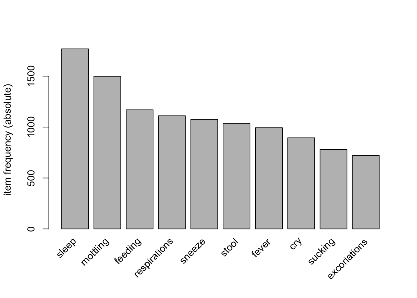

# Frequency Plots
itemFrequencyPlot(transactions,topN=10,type="absolute")

Frequent Itemsets

itemsets =  apriori(transactions, parameter = list(supp   = 0.03, 
                                                   conf   = 0.7,  
                                                   minlen = 3, 
                                                   target = "maximally frequent itemsets")
                    )

inspect(itemsets, by = "lift")

     items                           support    count
[1]  {excoriations, sleep, mottling} 0.03054049 152  
[2]  {cry, respirations, sucking}    0.03576452 178  
[3]  {cry, sleep, sucking}           0.04641350 231  
[4]  {sleep, sneeze, sucking}        0.03275065 163  
[5]  {sleep, respirations, sucking}  0.04098855 204  
[6]  {cry, sleep, fever}             0.03275065 163  
[7]  {sleep, sneeze, fever}          0.04139040 206  
[8]  {sleep, fever, respirations}    0.04560981 227  
[9]  {sleep, mottling, fever}        0.03475990 173  
[10] {cry, sleep, stool}             0.03154511 157  
[11] {sleep, sneeze, stool}          0.03335343 166  
[12] {sleep, respirations, stool}    0.03496082 174  
[13] {cry, sleep, feeding}           0.03134418 156  
[14] {cry, sleep, sneeze}            0.03737191 186  
[15] {cry, sleep, respirations}      0.05123568 255  
[16] {cry, sleep, mottling}          0.03596544 179  
[17] {sleep, sneeze, feeding}        0.03033956 151  
[18] {sleep, sneeze, respirations}   0.04741812 236  
[19] {sleep, mottling, sneeze}       0.03757284 187  
[20] {sleep, mottling, respirations} 0.03697006 184

Frequent Rules

# Generate and Prune ASSOCIATION RULES
rules <- apriori(transactions, parameter = list(supp = 0.01, 
                                               conf = 0.70, 
                                               minlen = 1, 
                                               maxlen = 5, 
                                               target = "rules")
                )
sortedRules <- sort(rules, by="lift", decreasing=TRUE)

summary(sortedRules)

set of 42 rules

rule length distribution (lhs + rhs):sizes
 3  4  5 
 5 36  1 

   Min. 1st Qu.  Median    Mean 3rd Qu.    Max. 
  3.000   4.000   4.000   3.905   4.000   5.000 

summary of quality measures:
    support          confidence        coverage            lift      
 Min.   :0.01005   Min.   :0.7033   Min.   :0.01125   Min.   :1.980  
 1st Qu.:0.01160   1st Qu.:0.7201   1st Qu.:0.01507   1st Qu.:2.027  
 Median :0.01366   Median :0.7489   Median :0.01849   Median :2.141  
 Mean   :0.01598   Mean   :0.7659   Mean   :0.02103   Mean   :2.234  
 3rd Qu.:0.01703   3rd Qu.:0.7865   3rd Qu.:0.02270   3rd Qu.:2.239  
 Max.   :0.03737   Max.   :0.9107   Max.   :0.04842   Max.   :4.078  
     count       
 Min.   : 50.00  
 1st Qu.: 57.75  
 Median : 68.00  
 Mean   : 79.55  
 3rd Qu.: 84.75  
 Max.   :186.00  

mining info:
         data ntransactions support confidence
 transactions          4977    0.01        0.7
                                                                                                              call
 apriori(data = transactions, parameter = list(supp = 0.01, conf = 0.7, minlen = 1, maxlen = 5, target = "rules"))

inspect(sortedRules[1:10])

     lhs                                   rhs            support    confidence
[1]  {respirations, sucking, feeding}   => {cry}          0.01105083 0.7333333 
[2]  {cry, fever, stool}                => {respirations} 0.01004621 0.7462687 
[3]  {cry, sneeze, fever, respirations} => {sleep}        0.01024714 0.9107143 
[4]  {cry, sneeze, fever}               => {sleep}        0.01547117 0.9058824 
[5]  {excoriations, cry, respirations}  => {sleep}        0.01205546 0.8955224 
[6]  {cry, mottling, sneeze}            => {sleep}        0.01326100 0.8684211 
[7]  {sneeze, fever, sucking}           => {sleep}        0.01366285 0.8607595 
[8]  {excoriations, cry, sucking}       => {sleep}        0.01084991 0.8437500 
[9]  {cry, sneeze, respirations}        => {sleep}        0.01928873 0.8205128 
[10] {excoriations, cry, mottling}      => {sleep}        0.01004621 0.8064516 
     coverage   lift     count
[1]  0.01506932 4.077989 55   
[2]  0.01346192 3.343096 50   
[3]  0.01125176 2.563702 51   
[4]  0.01707856 2.550100 77   
[5]  0.01346192 2.520936 60   
[6]  0.01527024 2.444645 66   
[7]  0.01587302 2.423077 68   
[8]  0.01285915 2.375194 54   
[9]  0.02350814 2.309781 96   
[10] 0.01245730 2.270198 50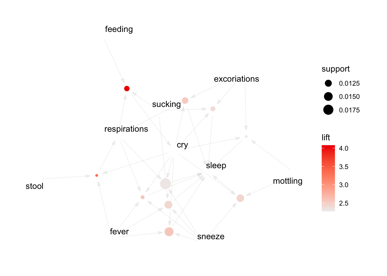

plot(sortedRules[1:10], method="graph")

Frequent Symptom Sequences

seqDB <- raw %>% mutate(sequenceID = bid, eventID = oid) %>%
          select(-c(tid, bid, oid, nas, num_items, tremors_disturbed, tremors_undisturbed, tone))
seqDB <- pivot_longer(seqDB, c(1:17) ) %>% filter(value > 0)

sequences <- seqDB %>%
  group_by(sequenceID, eventID) %>%
  summarize(
    SIZE = n(),
    items = paste(as.character(name), collapse = ';')
  )

`summarise()` has regrouped the output.
ℹ Summaries were computed grouped by sequenceID and eventID.
ℹ Output is grouped by sequenceID.
ℹ Use `summarise(.groups = "drop_last")` to silence this message.
ℹ Use `summarise(.by = c(sequenceID, eventID))` for per-operation grouping
  (`?dplyr::dplyr_by`) instead.

names(sequences) = c("sequenceID", "eventID", "SIZE", "items")
sequences <- data.frame(lapply(sequences, as.factor))
sequences <- sequences[order(sequences$sequenceID, sequences$eventID),]

write.table(sequences, "seqDB.txt", sep=";", row.names = FALSE, col.names = FALSE, quote = FALSE)
seq_mat <- read_baskets("seqDB.txt", sep = ";", info = c("sequenceID","eventID","SIZE"))

s1 <- cspade(seq_mat, parameter = list(support = 0.4, maxsize = 5), control = list(verbose = TRUE))
# PARAMETERS: 
# support: minimum support of a sequence (default 0.1).
# maxsize: (integer) max number of items of an element of a sequence (default 10).
# maxlen: (integer) max number of elements of a sequence (default 10).
# mingap: (integer) min time diff between consecutive elements of a sequence (default none, range >= 1).
# maxgap: (integer) max time diff between consecutive elements of a sequence (default none).
# maxwin: (integer) max time diff between any two elements of a sequence (default none.

s1.df <- as(s1, "data.frame")
summary(s1)

set of 30943 sequences with

most frequent items:
       sleep       sneeze        fever respirations        stool      (Other) 
       28271        17044        15417        11055         6928        15716 

most frequent elements:
       {sleep}       {sneeze}        {fever} {respirations}        {stool} 
         25124          14124          12874           8052           5980 
       (Other) 
         31648 

element (sequence) size distribution:
sizes
   1    2    3    4    5    6    7    8    9   10 
  75  818 3448 7437 8946 6422 2809  796  169   23 

sequence length distribution:
lengths
   1    2    3    4    5    6    7    8    9   10 
  13  199 1323 4560 8189 8931 5518 1806  369   35 

summary of quality measures:
    support      
 Min.   :0.4012  
 1st Qu.:0.4128  
 Median :0.4360  
 Mean   :0.4521  
 3rd Qu.:0.4709  
 Max.   :1.0000  

includes transaction ID lists: FALSE 

mining info:
    data ntransactions nsequences support
 seq_mat          4377        172     0.4

head(arrange(s1.df, desc(support)),30)

                                    sequence   support
1                                  <{sleep}> 1.0000000
2                          <{sleep},{sleep}> 0.9941860
3                  <{sleep},{sleep},{sleep}> 0.9651163
4                                 <{sneeze}> 0.9302326
5                                  <{fever}> 0.9127907
6                         <{sleep},{sneeze}> 0.9069767
7          <{sleep},{sleep},{sleep},{sleep}> 0.9069767
8                          <{fever},{sleep}> 0.9011628
9                         <{sneeze},{sleep}> 0.8953488
10                                 <{stool}> 0.8837209
11                <{sleep},{sleep},{sneeze}> 0.8779070
12                          <{respirations}> 0.8662791
13                         <{sleep},{stool}> 0.8662791
14                <{sneeze},{sleep},{sleep}> 0.8662791
15                 <{fever},{sleep},{sleep}> 0.8662791
16 <{sleep},{sleep},{sleep},{sleep},{sleep}> 0.8546512
17                                   <{cry}> 0.8430233
18                 <{sleep},{sleep},{stool}> 0.8430233
19                        <{fever},{sneeze}> 0.8430233
20                       <{sneeze},{sneeze}> 0.8430233
21                          <{sleep,sneeze}> 0.8372093
22                         <{stool},{sleep}> 0.8372093
23                <{sleep},{sneeze},{sleep}> 0.8372093
24         <{fever},{sleep},{sleep},{sleep}> 0.8313953
25                         <{sleep},{fever}> 0.8313953
26                  <{respirations},{sleep}> 0.8255814
27                  <{sleep},{respirations}> 0.8255814
28        <{sneeze},{sleep},{sleep},{sleep}> 0.8197674
29                           <{cry},{sleep}> 0.8139535
30        <{sleep},{sleep},{sleep},{sneeze}> 0.8081395

# Get induced temporal rules from frequent itemsets
r1 <- as(ruleInduction(s1, confidence = 0.9, control = list(verbose = TRUE)), "data.frame")
head(r1)

                                                                 rule   support
226         <{respirations},{sleep},{sleep},{sucking}> => <{sucking}> 0.4418605
266  <{respirations},{sleep},{respirations},{sucking}> => <{sucking}> 0.4011628
1338                                           <{stool}> => <{stool}> 0.7965116
1376                                   <{stool,sucking}> => <{stool}> 0.4011628
1436                                   <{stool},{stool}> => <{stool}> 0.7267442
1441                                     <{sleep,stool}> => <{stool}> 0.6279070
     confidence     lift
226   0.9156627 1.175328
266   0.9078947 1.165357
1338  0.9013158 1.019910
1376  0.9200000 1.041053
1436  0.9124088 1.032463
1441  0.9000000 1.018421

Quotes

Outline

Disclosure

Background of the Problem

Neonatal Abstinence Syndrome (NAS)

Finnigan NAS Score (FNASS)

Goal

Research Team

Background of the Method

Itemset & Rule Mining

Applications

Terminology

Measures of Strength and Interest

Example

Binary Database

Rule Mining / Itemset Selection

Aprior Algorithm

Compact representations

Compact representations (cont)

Compact Representation Diagram

R packages

R packages

Install and Load

aRules 1.7-5

Example

arulesViz 1.5-2

Frequent Sequences

Crux

Crux(es)

Symptom Mining

Symptom Mining

Frequent Itemsets

Frequent Rules

Frequent Symptom Sequences

`arulesViz` 1.5-2